We frequently need to compare data from different sources to identify discrepancies. If there is a large data set that requires more than eyeballing, it is better to know what functions in Excel that might help. It is easy to compare data of two values. After you identify the discrepancies, you can use either the “FILTER” command (“Data” tab on the ribbon → Filter) to filter out the only rows that have discrepancies or use the “Conditional Formatting” command to show the rows that have discrepancies.
If you have data in column A and B, you can either use the “=” or the DELTA function to do it. Below are the formulas:
=IF(A1=B1,”Match”,”Not Match”)
=IF(DELTA(A1,B1)=1,”Match”,”Not Match”)
The DELTA function returns “1” if the data in cell A1 and B1 are exactly the same. Please note that the DELTA function does not work with more than two numbers. In addition, it only compares numbers, not text. The “=” works with both numbers and text.
When you need to compare more than 2 values, the complexity gets in. Let’s look at the below example of comparing 3 values:

If I only need to know the match condition, I can input the below formula for cell E2 and copy such formula to cell E3 to E8.
=IF(AND(A2=B2,A2=C2,A2=C2),”Match”,”Not match”)
If I want to know more information like how many numbers deviate from the first number (leftmost number of my selection), I can use the below formula for cell G2:
=MAX(2-(DELTA(A2,B2)+DELTA(B2,C2)+DELTA(C2,A2)),0)
- If all 3 numbers on the same row are the same, the sum of the DELTA functions returns 3. I put a MAX to zero condition to avoid the result showing as a negative number.
- If 1 number on the same row is different from the other 2 numbers, the sum of the DELTA functions returns 1. Please look at row 4 at the above example, Value 3 (1.000000) is the only value that is different from the other 2 values (0.972002). So the DELTA function of A4 vs. C4 and B4 vs. C4 will both return 0 while only A4 vs. B4 will return 1. By using 2 to subtract the sum of DELTA functions, it will return 1 and shows that there is one value that deviates from the others.
- If all 3 numbers on the same row are different, the sum of the DELTA functions returns 0. So 2 minus 0 will be 2 and that shows 2 values deviate from the leftmost column of my data selection.
The complexity increase substantially when you have to compare more than 3 values. If there are 4 values to compare, you need to put in:
=IF(AND(A2=B2,A2=C2,A2=D2,B2=C2,B2=D2,C2=D2),”Match”,”Not match”)
Please note that the number of comparison combination (within the “AND” function) is now 6. The number of the comparison combination grows like this:

When you have many numbers to compare, you can consider the below two methods to do so. Each method has its own shortcoming, but can save you some time if you just want to do a quick comparison.
Use “GO TO” commands in Excel
Step 1: Highlight the cells that you want to check the discrepancies.
Step 2: Press “F5” to initiate the GO TO command.
Step 3: Click the “Special…” button.


Step 4: Choose “Row difference” and then click “OK” to confirm your selection

Now you should see the cells that are highlighted (cell B3, B4, and C4). The values in the highlighted cells are different from the leftmost column of your selection (in this example, column A).
The shortcoming of this method is that the highlight is not permanent. Once your click your mouse, the highlight is gone. However, it is good for quick spot of small dataset and this method is applicable for both numbers and text.
Use AVERAGE function to compare
This method only works for numbers, not text. If the average of all numbers that you want to compare is the same as the first number, the chance is that all numbers are the same is very high. Of course, you need to take the risk that some numbers on the same row may even out themselves. Since you are the one who knows about your data, you can judge it yourself if this method is valid for your usage. The formula in the below screenshot is:
=IF(AVERAGE(A2:D2)=A2,”Match”,”Not match”)