Count duplicates as one item

Requirement: Knowledge of Excel Array Functions
File to download: None
Related articles: Data Transposing
I have a list of duplicate entries as shown in the left picture. There are 19 entries altogether with duplicates. For example, China in the list appears 4 times. For reporting purposes, I am only interested in the number of countries, regardless of duplications. In this example, the number of individual countries are 7 (China, USA, Philippines, Malaysia, Russia, France, and Germany).
There are several ways of doing it:
1. You can use “Filter” and manually count the list of filtering. Well, we want to stay away the manual counting part.
2. You can also use pivot table to see the number of countries and manually count it. Besides the manual counting work, pivot table requires manual refreshing every time you update the data.
3. If you know the list of the individual countries, you can use the COUNTIF function to list it. However, it defeats the purpose of this project because we don’t know the number of individual country and that is why we want to count the list.
In addition, if we need to run a report for this purpose on a frequent basis, none of the above way will work well.
Microsoft Excel has a nice way of doing it by using one of the array functions. Excel borrows the data manipulation concept from databases and has its own set of array functions. All the array functions require you to press CTRL + SHIFT + ENTER on your keyboard at the same time to enter such functions. The formula in the cell will appear to be enclosed by {}.
To achieve our goal, the formula to be used will be:
=SUM(1/COUNTIF(A1:A19,A1:A19)) and then press (CTRL + SHIFT + ENTER) all 3 keys at the same time instead of just the ENTER key. The formula will then be enclosed by brackets like this: {=SUM(1/COUNTIF(A1:A19,A1:A19))}
The formula can be entered anywhere other than cell A1 to A19. The formula does not look intuitive and needs some explanations.
1. The COUNTIF function counts the data against itself. The range and criteria in the COUNTIF function are exactly the same. They both are the range of data set in our example (cell A1 to A19). The result is China occurs 4 times, USA occurs 3 times, Philippines occurs 2 times, …, etc. Please note that this is an array function, so there is not one result. There are 7 results in this case. If you just enter =COUNTIF(A1:A19,A1:A19) in the cell without using the CTRL+SHIFT+ENTER keys, it will only give you one of the 7 results.
2. We want the same duplicates counted as just one. For example, China shows up 4 times, but we want it counted as one. That is how the 1 divided by occurrence come in place. For China, 1 divided by 4 will become 0.25. Since China occurs 4 times, so 4 times 0.25 will come back to 1. So China is counted as one even though it occurs 4 times on the list. Same logic applies to other countries. For another example, USA occurs 3 times, so 1/3 equals 0.33333 and 3 times 0.33333 will become 1. The SUM function will sum up such results for all countries (each country will be counted as one) and tells you that there are 7 countries in the list.
The array function works wonder in this example. No manual counting and refreshing is required. Every time you update the list, the formula will automatically return the unique count result. Nice and beautiful !